ggsmatr example • ggsmatr

library(ggsmatr)
#> 
#> 
#> ##~~~~~~~~~~~~~~~~~~~~~~~~~~~~~~~~~~~~~~~~~~~~~~~~~~~~~~~~~~~~~~~~~~~~~~~~~~~~~~
#> ##                            ggsmatr - R package                         ----
#> ##~~~~~~~~~~~~~~~~~~~~~~~~~~~~~~~~~~~~~~~~~~~~~~~~~~~~~~~~~~~~~~~~~~~~~~~~~~~~~~ 
#> 
#> El paquete ggsmatr se ha cargado con éxito. ¡Espero que lo disfrutes!
#>  Email de contacto: sandoval.m@hotmail.com 
#> Para citar este paquete: Mario A. Sandoval-Molina (2023). ggsmatr: a simple and efficient way to visualize the coefficients of the (Standardized) Major Axis Estimation fit. R package version 0.1.
library(ggplot2)
library(smatr)
#> Warning: package 'smatr' was built under R version 4.6.1

ggsmatr: Example using the iris dataset

The presence of fitted SMA lines in a ggplot2 scatter plot can be obtained from an object created with smatr::sma(). We first read the example data included in the package and we fit a common-slope SMA by group.

datafile <- system.file("iris.csv", package = "ggsmatr")
df.iris <- read.csv(datafile, encoding = "UTF-8")

fit <- sma(
  Sepal.Length ~ Sepal.Width + Species,
  data = df.iris,
  shift = TRUE,
  elev.test = TRUE,
  alpha = 0.05
)

ggsmatr(
  data = df.iris,
  groups = "Species",
  xvar = "Sepal.Width",
  yvar = "Sepal.Length",
  sma.fit = fit
) +
  theme(legend.position = "top", legend.title = element_blank()) +
  ylab("Sepal.Length") +
  xlab("Sepal.Width")
#>        group    r2  pval
#> 1     setosa 0.551 0.000
#> 2 versicolor 0.277 0.000
#> 3  virginica 0.209 0.001
#> Warning: Using `size` aesthetic for lines was deprecated in ggplot2 3.4.0.
#> ℹ Please use `linewidth` instead.
#> ℹ The deprecated feature was likely used in the ggsmatr package.
#>   Please report the issue to the authors.
#> This warning is displayed once per session.
#> Call `lifecycle::last_lifecycle_warnings()` to see where this warning was
#> generated.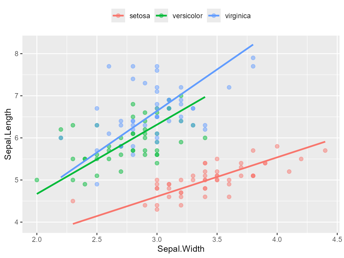

Confidence ribbons for SMA slopes

Given that SMA lines pass through the group centroid, the presence of a parametric confidence ribbon can be added with ci = TRUE. The ribbon is related with the slope confidence intervals already stored in the sma() fit (Slope_lowCI and Slope_highCI), and it is not related with the OLS band of geom_smooth().

The confidence level is the one used when the model is fitted, for example sma(..., alpha = 0.05) for 95% intervals. According to Warton et al. (2006, 2012) those limits are obtained by inverting the one-sample test for the SMA slope, and ggsmatr() only maps them onto the plot.

Because the fitted line is constrained to pass through the group mean (xbar, ybar), slope and intercept are not independent. The presence of a slope interval is therefore converted to a family of lines through the same centroid:

y_low  <- ybar + Slope_lowCI  * (x - xbar)
y_high <- ybar + Slope_highCI * (x - xbar)
ymin   <- pmin(y_low, y_high)
ymax   <- pmax(y_low, y_high)

pmin() and pmax() are required, because the lower slope produces the higher line when x < xbar. The envelope pinches at the group mean and fans out toward the ends of the observed x range. This presents a slope-CI envelope, not a bootstrap prediction band and not a pointwise CI for E[Y | X].

The numerical intervals can be inspected in the smatr object:

fit$groupsummary[, c("group", "Slope", "Slope_lowCI", "Slope_highCI")]
#>        group    Slope Slope_lowCI Slope_highCI
#> 1     setosa 0.929894   0.7665449     1.128053
#> 2 versicolor 1.644914   1.2882605     2.100306
#> 3  virginica 1.971740   1.5274522     2.545258

ggsmatr(
  data = df.iris,
  groups = "Species",
  xvar = "Sepal.Width",
  yvar = "Sepal.Length",
  sma.fit = fit,
  ci = TRUE
) +
  theme(legend.position = "top", legend.title = element_blank()) +
  ylab("Sepal.Length") +
  xlab("Sepal.Width")
#>        group    r2  pval Slope Slope_lowCI Slope_highCI
#> 1     setosa 0.551 0.000 0.930       0.767        1.128
#> 2 versicolor 0.277 0.000 1.645       1.288        2.100
#> 3  virginica 0.209 0.001 1.972       1.527        2.545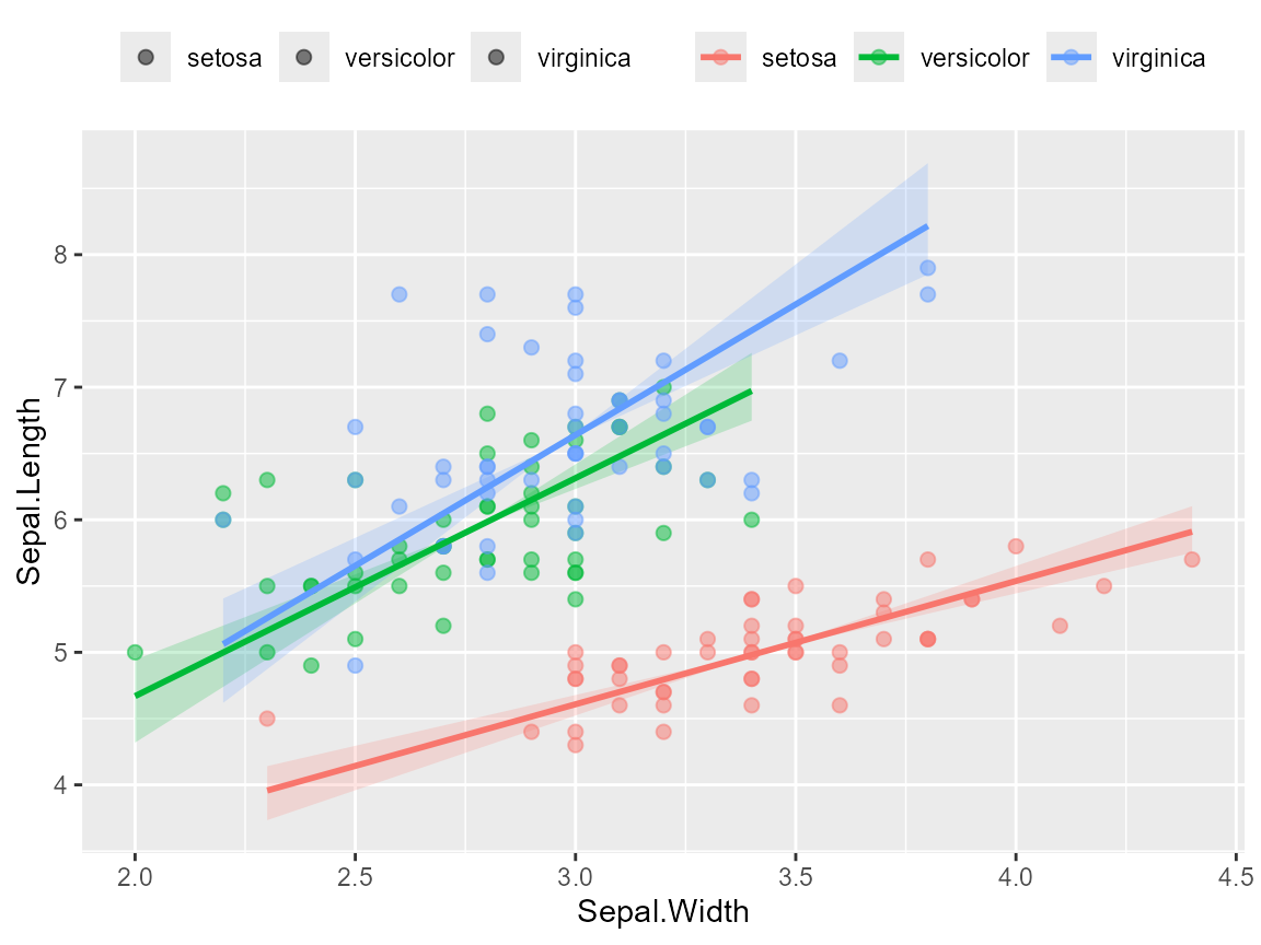

Transparency and smoothness of the ribbon can be controlled with ci.alpha and n:

ggsmatr(
  data = df.iris,
  groups = "Species",
  xvar = "Sepal.Width",
  yvar = "Sepal.Length",
  sma.fit = fit,
  ci = TRUE,
  ci.alpha = 0.15,
  n = 150
)

References

Warton, D. I., Wright, I. J., Falster, D. S. and Westoby, M. (2006). Bivariate line-fitting methods for allometry. Biological Reviews 81, 259–291.

Warton, D. I., Duursma, R. A., Falster, D. S. and Taskinen, S. (2012). smatr 3 – an R package for estimation and inference about allometric lines. Methods in Ecology and Evolution 3, 257–259.