Ggsmatr

An elegant extension of the smatr R package that leverages the ggplot2 interface to create beautiful, publication-ready plots.

Overview

ggsmatr brings together the power of standardized major axis (SMA) regression from the smatr package and the rich, customizable visualization capabilities of ggplot2. With just a few lines of code, you can generate clean, grouped scatter plots with fitted SMA lines and optional parametric confidence ribbons — perfect for exploratory analysis and scientific publications.

Installation

Make sure you have the required dependencies installed, and then install ggsmatr from GitHub:

install.packages(c("ggplot2", "smatr"))

# install.packages("devtools")
devtools::install_github("mariosandovalmx/ggsmatr")

Quick Start

Here’s a complete example using the classic Iris dataset.

1. Load the data

datafile <- system.file("iris.csv", package = "ggsmatr")
df.iris  <- read.csv(datafile, encoding = "UTF-8")

2. Load the libraries and fit the SMA model

The confidence level of the ribbon is the one used in sma(), for example alpha = 0.05 for 95% intervals.

library(ggsmatr)
library(ggplot2)
library(smatr)

fit <- sma(
  Sepal.Length ~ Sepal.Width + Species,
  data      = df.iris,
  shift     = TRUE,
  elev.test = TRUE,
  alpha     = 0.05
)

3. Build the plot

ggsmatr(
  data    = df.iris,
  groups  = "Species",
  xvar    = "Sepal.Width",
  yvar    = "Sepal.Length",
  sma.fit = fit
) +
  theme(
    legend.position = "top",
    legend.title    = element_blank()
  ) +
  ylab("Sepal.Length") +
  xlab("Sepal.Width")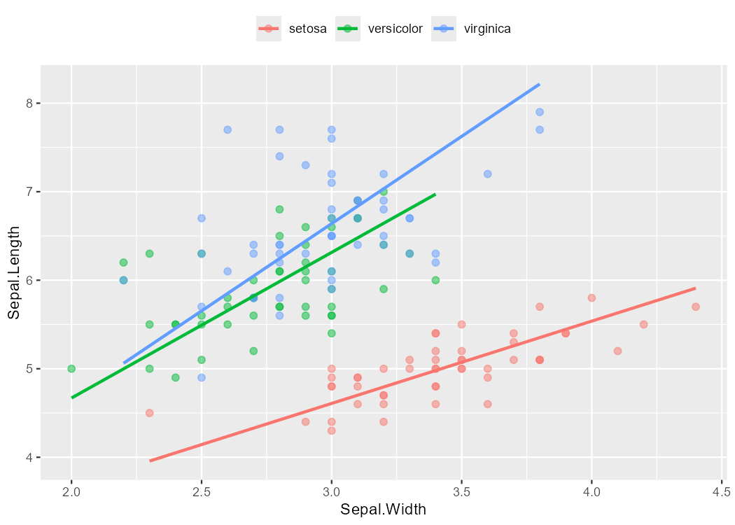

Grouped SMA plot for iris sepal width and sepal length

4. Add a parametric confidence ribbon

SMA is not OLS, so geom_smooth(se = TRUE) is not related with the intervals stored in the smatr fit. Set ci = TRUE to draw a slope-CI envelope pivoted at each group centroid:

ggsmatr(
  data    = df.iris,
  groups  = "Species",
  xvar    = "Sepal.Width",
  yvar    = "Sepal.Length",
  sma.fit = fit,
  ci      = TRUE
) +
  theme(
    legend.position = "top",
    legend.title    = element_blank()
  ) +
  ylab("Sepal.Length") +
  xlab("Sepal.Width")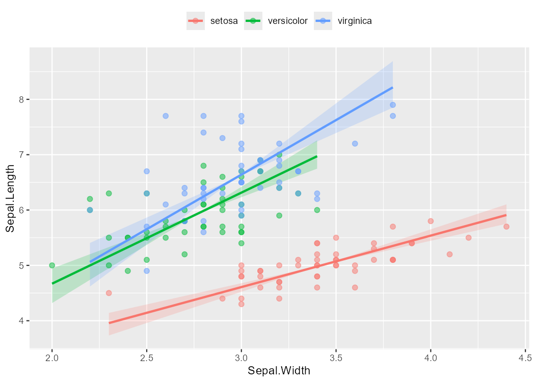

Grouped SMA plot with parametric slope confidence ribbons

How the confidence ribbon is calculated

The ribbon is not an OLS interval from geom_smooth(se = TRUE), and it is not obtained by combining intercept CIs with slope CIs independently. SMA (and MA) lines are constrained to pass through the group centroid $(\bar{x}, \bar{y})$ , so slope and intercept are related with each other: the elevation is $\bar{y} - b\,\bar{x}$ .

smatr::sma() already constructs confidence intervals for the slope by inverting the one-sample slope test (Warton et al. 2006, 2012). Those limits are stored in sma.fit$groupsummary as Slope_lowCI and Slope_highCI. The confidence level is the one used when the model is fitted, for example sma(..., alpha = 0.05) for 95% intervals.

Given the presence of a fitted SMA line through the centroid, ggsmatr() maps that slope interval to a family of lines through the same point. For each group and each $x$ along the observed range:

$y_{\mathrm{low}} = \bar{y} + b_{\mathrm{low}}(x - \bar{x}), \qquad y_{\mathrm{high}} = \bar{y} + b_{\mathrm{high}}(x - \bar{x})$

ymin and ymax are then taken with pmin() / pmax(), because the lower slope produces the higher line when $x < \bar{x}$ . The resulting envelope pinches at the group mean and fans out toward the ends of the line. Users can inspect the numerical intervals with:

fit$groupsummary[, c("group", "Slope", "Slope_lowCI", "Slope_highCI")]

What the ribbon presents is therefore a parametric slope-CI envelope. It does not include a separate intercept band, it is not a bootstrap prediction interval, and it is not a pointwise CI for $E[Y \mid X]$ as in ordinary least squares.

The ribbon can be tuned with ci.alpha (transparency) and n (number of x values evaluated in each group):

ggsmatr(
  data     = df.iris,
  groups   = "Species",
  xvar     = "Sepal.Width",
  yvar     = "Sepal.Length",
  sma.fit  = fit,
  ci       = TRUE,
  ci.alpha = 0.15,
  n        = 150
)

Features

Seamless integration with ggplot2 — chain any layer or theme you like.
SMA regression lines drawn automatically from a smatr::sma() fit.
Parametric confidence ribbons for the SMA slope, using the smatr slope CIs pivoted at each group centroid.
Group-aware plotting with consistent color mappings across points, lines and ribbons.
Fully customizable — labels, themes, legends, and more.

Package	Purpose
`smatr`	Standardized Major Axis regression
`ggplot2`	Grammar-of-graphics plotting
`ggsmatr`	The bridge between the two

Citation

If you use ggsmatr in your work, please cite the software. The preferred citation is the Zenodo DOI, which allows citation tracking:

citation("ggsmatr")

Sandoval-Molina, M. A. (2026). ggsmatr: ggplot2 based plots for (standardised) major axis estimation (R package version 0.2.0). https://doi.org/10.5281/zenodo.22737761

The source code is available at GitHub.

License

Released under the MIT License.

References

Warton, D. I., Wright, I. J., Falster, D. S. and Westoby, M. (2006). Bivariate line-fitting methods for allometry. Biological Reviews 81, 259–291.

Warton, D. I., Duursma, R. A., Falster, D. S. and Taskinen, S. (2012). smatr 3 – an R package for estimation and inference about allometric lines. Methods in Ecology and Evolution 3, 257–259.